Data Science Projects

This data was given to my team and I from the ABA

The goals of the ABA are to promote the platform to low-income clients, recruit new attorneys, train these attorneys, and improve the overall user experience. Our overall goal is to relate the category of the client’s question to their age, geographic region, and ethnic identity to detect trends or patterns. This can help train attorneys to be more efficient in their responses. Another goal is to identify categories that have areas of need in terms of response rates. By identifying these areas of need, we can offer better recommendations as to where the ABA should allocate its resources to maximize efficiency.

This data contained a lot of different information that we could use to create our analysis, We condensed the amount of different data by separating states in regions to get a better look and create better visualizations about the clients. My team dedicated most of our time to recruiting and preparing new attorneys. To do so we looked at the type of clients in certain areas and the questions these clients were asking in certain areas. Some of the most asked questions included, Houses and Homelessness, Family and Children, and Consumer Financial. Using some statistical techniques we were able to create some visualizations to help show lawyers where they should spend the majority of their time. The first one we created was a line graph that shows the questions asked by year.

In this graph, as I said above you can see the dramatic increase in Family and Children, Housing and Homelessness, and in this case, Other which were topics we did not have access to.

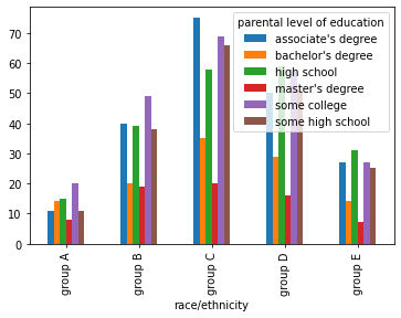
This next graph was created to show lawyers what cases are most popular in their location. The three main ones were obviously present in all locations but we made this for the exact reason of spotting things such as the individual rights were predominantly shown in the southwest region.

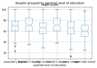
This graph shows the average duration of cases by category of case, so for the first time in one of our plots Family and Children were not the highest and neither was Housing and Homelessness. We found that Juvenile cases are the cases with the longest completion time followed by Consumer Financial Questions. This could be because it takes a lot longer for things to get approved in a Juvenile involved case, which shows lawyers that they need to prepare in advance that certain cases can and will take longer than others.

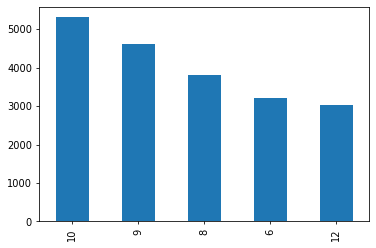
The final graph we made was the percentage of questions unanswered by category, We made this graph to show lawyers where they could find the most available and needed work. Back at the top again was the Juvenile category which had around 42% of cases left unanswered. Followed by Individual Rights, which we thought could be because it is a risk-taking one of these cases because lawyers know how much harder it is to legally do things while representing a juvenile, and representing rights cases can also be a lot harder than an Education case in some instances.

One potential solution to improve the quality of legal assistance and client understanding is to provide comprehensive training programs for new attorneys. By equipping attorneys with the necessary skills and knowledge, they can better serve their clients and provide more effective legal representation.

As for the data analysis, our findings suggest that there is a high demand for Family and Children attorneys, as evidenced by the high number of unanswered questions in that category. If the data were to be resampled in the future, we would expect to see a decrease in the number of unanswered questions in this category due to the increased availability of qualified attorneys.

Additionally, we found that the juvenile category had the highest number of unanswered questions, which we attribute to the lengthy nature of juvenile trials. To address this issue, it may be beneficial to streamline the juvenile court process or allocate additional resources to improve efficiency and reduce the time it takes to resolve these cases. By training attorneys to specialize in these categories the ABA will be able to increase access to such a critical resource.

For this reflection I read and analyzed a dataset about penguins in Antartica which can be found here: https://www.kaggle.com/datasets/parulpandey/palmer-archipelago-antarctica-penguin-data

The Objective of this assignment was to make a KNN classifier with different ranges of k values from 1 – 40 and find the best one and the mean f1 score for each of the K lengths. To start like any other KNN classifier I split the data between Tain and Test for both of them I used the StandardScaler library from Sklearn to transform the data and set the number of KNeighbors to the value of k which in this case iterates from 1 – 40. For the Test function I split the test data and also called StandardScaler on the data to transform it, additionally one of the difference between Test and Train is making a predictions array in test to hold all of my prediction values to later evaluate my predictions to the actual values.

Within the KNN function I pass in the k value, the data-frame, the features which to use to predict, and the target value. In this case my features were culmen depth in mm and the flipper length in mm and the target value to predict was the island for which the penguin resided. The KNN function is essentially just a for loop that iterates through the train and test index and calls the test function on the true verse predicted values which will return a prediction. That prediction along with the true values are passed into the evaluation function which calculates the f1 score which combines precision and recall to determine the accuracy of the predictions made. As I said above I would be finding the mean of these f1 scores so also within the KNN function I kept and a variable assigned to the evaluation function to hold that f1 score and stored them in an array after each run then after the loop I took the mean of the f1 scores. Now to figure out the best ‘K’ value I created a list of k-values 1 -40 and made a for loop to run the KNN function but increasing the k-value by one each time and running ten k-folds each. After each run the loop compares scores to store the highest one and at the very end prints the best k and prints the best f1 score.

Here is an output example

KNN for k = 1 is: 0.6447385428322892
KNN for k = 2 is: 0.6096944091093646
KNN for k = 3 is: 0.587228533127487
KNN for k = 4 is: 0.6329413513901605
KNN for k = 5 is: 0.6399729864160182
KNN for k = 6 is: 0.6173035863111862
KNN for k = 7 is: 0.6479615526860656
KNN for k = 8 is: 0.6559180911112491
KNN for k = 9 is: 0.6355883552135018
KNN for k = 10 is: 0.6367094597526258
KNN for k = 11 is: 0.6601321836835505
KNN for k = 12 is: 0.6874331167593228
KNN for k = 13 is: 0.673744989312876
KNN for k = 14 is: 0.65714994642037
KNN for k = 15 is: 0.6587411579652839
KNN for k = 16 is: 0.6509181156347517
KNN for k = 17 is: 0.6773768997965366
KNN for k = 18 is: 0.6730539237034099
KNN for k = 19 is: 0.6763714345274077
KNN for k = 20 is: 0.6736193550832233
KNN for k = 21 is: 0.6685218227558851
KNN for k = 22 is: 0.6802164940267407
KNN for k = 23 is: 0.6828297467048432
KNN for k = 24 is: 0.6755306619112366
KNN for k = 25 is: 0.6778217033972156
KNN for k = 26 is: 0.6825008768259028
KNN for k = 27 is: 0.6798186745498981
KNN for k = 28 is: 0.6689349852542978
KNN for k = 29 is: 0.6784235175815404
KNN for k = 30 is: 0.6878112656848122
KNN for k = 31 is: 0.6863575370058603
KNN for k = 32 is: 0.6875116682480806
KNN for k = 33 is: 0.6768914742286175
KNN for k = 34 is: 0.6755678601425782
KNN for k = 35 is: 0.6842258588233825
KNN for k = 36 is: 0.6824704306576266
KNN for k = 37 is: 0.6812679573836695
KNN for k = 38 is: 0.6880329625844984
KNN for k = 39 is: 0.6882488474406613
KNN for k = 40 is: 0.675187658176038
The best value for k is: 39
The best f1 score is: 0.6882488474406613

So this means the best k-value for this run was 39 which means the highest mean f1 score was when the number of KNeighbors for the KNN classifier was at 39.

In this post I am going to be comparing seven categorical features that I recoded from the dataset, to try and get the highest precision, recall, f1, accuracy, and prediction scores. I will make a confusion matrix to show the most accurate prediction for each level, so for the highest values with one feature then two and so on. I got this dataset from kaggle originally and recoded the numeric columns to their equivalent categorical. Going into this I am expecting that the course_cat and gender columns will impact the scores the highest since the course column has a wide range of classes and the gender should give a good split on the data.

https://www.kaggle.com/datasets/thedevastator/higher-education-predictors-of-student-retention

My highest one value alone was the course_cat column which was the columns that had the courses the student was enrolled in, here are the values and confusion matrix for that column. Considering looking that the predictor got 64% F1 for just one feature that is a very good feature since there is over 35 features in the whole dataset that means the course the student was in has a very high rate by itself.

Accuracy: 0.6859504132231405
F1-score: 0.6443150513398449
Average precision: 0.6533690114823829
Average recall: 0.6553719008264463
Average F1 0.6227310408979837

Looking at my confusion matrix I got 453 True Positive values, 968 False Positive, 283 False Negatives, 1926 True Negative

Next I compared every other feature to the course feature and found that course and scholarship together were the highest among them all, here are the values and confusion matrix of that one. The scholarship column and course column together added to be the second highest value of an F1 of 73%, while the other columns actually brought the predictor down, which is probably because the gender for example didn’t have the best matchup with the course column.

Accuracy: 0.7355371900826446
F1-score: 0.7368317632780442
Average precision: 0.6986419399259287
Average recall: 0.6977961432506886
Average F1 0.6972558024858767

Here there is 854 True Positives, 567 False Positives, 530 False Negatives, and 1679 True Negatives

For the three features Nationality ended up being the third feature that added the highest prediction value, here are the values and the confusion matrix for that set. Now the Nationality column can come into play with the course column and the scholarship column, which as I said above most likely means that the Nationality column and scholarship column went hand and hand because the F1 stayed relatively the same here at 73.3 while it went down for every other column mixed with course and scholarship.

Accuracy: 0.7327823691460055
F1-score: 0.7333657712947298
Average precision: 0.6965661008102548
Average recall: 0.6975206611570248
Average F1 0.696732808466049

Here there is 839 True Positives, 582 False Positives, 527 False Negatives, and 1682 True Negatives

My next highest prediction value was for course, scholarship, nationality, and gender here are the values and the confusion matrix for that. Adding gender made the accuracy go down a little bit to 70.2 , which I have my theory as to why is because the gender and nationality are not using each other as good as I thought they would, this is normal though it is common for the confusion matrix and f1 to go down slightly not every column will always make a positive difference.

Accuracy: 0.7079889807162535
F1-score: 0.7027808573540282
Average precision: 0.6985773751464521
Average recall: 0.7030303030303031
Average F1 0.6983946991748324

Here there is 785 True Positives, 636 False Positives, 442 False Negatives, and 1767 True Negatives

The next highest value was the displaced feature so we are now up to five features here’s the updated values and confusion matrix. The next highest addition was adding the displaced column which actually brought it even lower since the last one which is normal but we are now at 67% F1 so still right now the best combinations are with just two features which is a little shocking but thinking about what we are trying to find courses and scholarships make sense to be some of the highest values.

Accuracy: 0.6721763085399449
F1-score: 0.6713546502310838
Average precision: 0.7056193983805967
Average recall: 0.7074380165289256
Average F1 0.7049748102390314

Here there are 834 True Positives, 587 False Positives, 475 False Negatives, and 1734 True Negatives

The 6th feature being added is now the marital status of the student and with these 6 columns here are my values and the confusion matrix. Now this is starting to increase again from where we just were back up to 70% f1 with the addition of the marital status. Which I thought would’ve been added before now possibly the 3rd or 4th best feature but having it at 6th gives the highest accuracy.

Accuracy: 0.7079889807162535
F1-score: 0.7004894774432254
Average precision: 0.7011525271148762
Average recall: 0.7019283746556473
Average F1 0.6999156289535691

Here there are 831 True Positives, 590 False Positives, 492 False Negatives, and 1717 True Negatives

Now since we have compared all of them the 7th must be attendance so let’s see the final prediction values I got. Now with all seven values that are the highest amongst each other I see that we are at 72.8% F1, which is not the highest but it still has made its way back up to where it was.

Accuracy: 0.7272727272727273
F1-score: 0.7288041880764838
Average precision: 0.6928300955320715
Average recall: 0.6950413223140497
Average F1 0.6926414223613386

Here there are 811 True Positives, 610 False Positives, 497 False Negatives, and 1712 True Negatives

Overall, my highest percentage predictor was with course and scholarships at 73.6% F1 which looking back at my previous analysis on this dataset with only 2 columns being used but calculating it using naive bases algorithm and more of a probability approach I got right around the same percentage accuracy in both. I would like to continue analysis on this dataset and hope to fix some of the unstable columns with a lot more broad information and see how high I can really get this F1 and Accuracy I would feel very good getting it to 90% which I believe is very possible for this data.

The car dataset was found on Kaggle https://www.kaggle.com/datasets/lepchenkov/usedcarscatalog

For this assignment the first dataset I analyzed was hotel reservations, the first probability I looked at was P(Canceled) which was 32.76%. Or there is a 32.76% chance of a hotel reservation canceling. Next was P(Canceled, Not selected meal plan) so the probability that they canceled and did not select a meal plan is 4.68%. The probability they canceled out of the not selected meal plan group is 0.331%. Next, I analyzed the market segment type or why are they staying at the hotel. First was the probability they canceled their reservation out of the corporate group or work travel group over the canceled is 0.018%. The probability they are staying at the hotel for free or complementary out of the canceled group is 0%… makes sense.

Now to the other dataset which was on vehicles. I chose this dataset because of the interesting features like color, transmission type, and car brand. I was curious to see which of the car types had higher percentages of being a certain transmission type. First I wanted to see the probability of a car being diesel because it’s black which was found to be 0.195%. On the contrary, I tested the probability a car was gasoline because it was blue which is 0.149%. My next set of probabilities is on the make of the car. Firstly what is the probability of a car being mechanical because it is a Toyota, which is 0.025%, and a car being automatic if it is a honda has a probability of 0.0310% both of which I thought to be very low? I suppose a lot of Toyotas are automatic cars. Next was if the car had a warranty based on if it was new or owned. The probability of a car having a warranty if it is new was 0.856% and the probability of a car not having a warranty because it was previously owned was 0.998% therefore the probability of a used car having a warranty was 0.00196%, so concluding used cars do not have a warranty over 99% of the time and new cars do have a warranty 85% of the time.

In this assignment, I chose a dataset on exam scores of students with data such as ethnicity, parental education, lunch preference, whether or not they did test preparation, and the scores on three standardized tests. This is the site from which I found the data, https://www.kaggle.com/datasets/whenamancodes/students-performance-in-exams?resource=download.

The questions I wanted to answer.

Overall did more students pass or fail? Did the ones who completed the test review gain an advantage? Was there any significance between the students’ average test scores and their lunch opportunities, Did students of parents with higher education have an advantage on math exams? Does gender affect writing scores?

To begin solving my first question did the students who did the test review gain an advantage? To begin I added all the tests for each student to get their average of the three tests and if the average was over or equal to 60% that is considered a pass below is a fail. The frequency of the pass-fail was 713 passes and 287 fails. I then compared this to the number of students that completed the test preparation course. Here is that graph.

My next question was if there was any significance between the student’s average test scores and their lunch opportunity. To do so I used the other column I made which was the percentage of the student’s total test average compared to the two lunch options given free/reduced versus standard. Before running my test to see if it was even worth testing I created a notched box plot.

To run the T-test I made two separate arrays of the test scores separated by each lunch and ran them against each other getting a p-value of 3.18*10^-29. Seeing as this is way below 5% I was able to conclude that there is significance between which lunch students ate versus their average test scores.

The next question I wanted to figure out was if there are any big differences between race/ethnicity and the parental education of the students, here is what I found.

Another test I wanted to run was the math scores of students with parents with a master’s degree versus the parents with only some high school. Before doing so again I made a boxplot of all the parent’s education versus math scores and got this.

Another relationship I wanted to see was if there were any similarities in the writing versus reading test scores based on gender. Since these are both numeric values I made a scatter plot to show them versus each other. Here is what I found.

Now I decided to run a T-test on the data set of males versus females on writing scores and came out with a P-value of 2.96*10^-15 concluding that there is the significance that females tend to do better. One thing I noticed was that this was the highest or closest to 0.05 P-value of all my tests, if I had to guess it is because declaring something like this is significantly based on gender is hard to say whether it is correct or not. In the future running this on a bigger dataset would be beneficial.

Overall by choosing this data set I was able to analyze and predict a lot of new things when it came to students possibly receiving better test scores. I concluded that reviewing the test practice gave the student a much higher chance of receiving a better score than not doing it. I was able to see that free/reduced lunch versus standard lunch also had significance in receiving a better test score. I also ran a test to compare students with parents who had received a master’s degree verse kids with parents of only some high school education and compared those to the student’s scores on the math tests, because often when a student is struggling in math the first person they go to is their parents. I found that there was significance between the two parents’ education and the student’s math scores. I also compared writing versus reading scores based on gender in the form of a scatter plot and was able to conclude that females had higher test scores in both sections of the test, which is what I predicted because women tend to be better writers. In the future, I would like to test gender on writing scores with a bigger dataset, I would like to compare parental education to all test scores individually, I would like to have more columns such as was the student and athlete or possibly build a generator to add in if the student was an athlete at random. I also think adding more to the columns would help prove the statistical tests more right or wrong such as adding in if the student packed lunch.

I chose this dataset because I found comparing if someone cancels their hotel reservation to the month, meal plan, etc very interesting. Overall this analysis I found a few things that I believe correlate some columns to if someone will cancel or stay with their reservation. The dataset I found was on Kaggle (https://www.kaggle.com/datasets/ahsan81/hotel-reservations-classification-dataset). I observed a lot in this dataset and found a lot of things interesting such as The fact that the fall months had the most reservations personally was expecting a summer month to be the highest, but I do understand traveling to more scenery-based places like the mountains is very common. I also found the difference in cancel verse non-cancel was about 75% compared to 25%. I did notice on the heatmap that although October had the highest reservations its balance of cancel to not canceling was close at around 3,500 showing and 2.500 not. Although in another month say December there were around 2.500 non-cancels and only around 400 cancels, assuming because a lot of people are visiting family and have some big priorities when it comes to travel.

In conclusion, I can conclude that the highest month for hotel reservations will be October in both cancelation and non-cancelation, as for any month whatever months have the higher total reservations will most likely have a higher canceling rate but also a non-canceling rate.

Welcome to Sites@UMW. This is your first post. Edit or delete it, then start writing!